CauseF manual (v. 5.0)

Contents

Overview
Default settings - Set default options for all modules
Grid - Key points, Settings window, Grid window
Spheres - Key points, Settings window, Spheres window
Planets - Key points, Settings window, Planets window
Bones - Concept, Process, Key points, Settings window, Bones window, Bones properties window, Presets, Tips and hints
Contact and bug report
Copyright and credits, references, history

 

Grid

Key points
Settings window
Grid window

Key points

You can
- select the number of functional elements, from a minimum of 100 to as many as your system's memory allows (even something like 700,000 and upwards);
- select the number of sources that are meant to transmit to the rest of the elements;
- divide the sources and/or the rest into regions;
- select the probability levels for each region;
- select static probability levels or allow them to self-adjust as the system keeps cycling and thereby changes the activation levels for the individual elements;
- select cycle limits - overall, consecutive increments, or when a particular activation level has been reached;
- observe the effects across the whole system as clusters form and view their changing activation levels as they send and receive, given the selected criteria;
- use CauseF to simulate real-world scenarios, such as the spreading of a disease across a population under various conditions, having carriers, recipients, mitigating and/or exacerbating influences acting on the members and/or regions. Any scenario can be simulated provided its definitions can be transposed across to CauseF meaningfully (a most crucial point when it comes to models per se: unless a model has at least some relationship to the real it is useless).

But generally, observe how in such a system the range of probable outcomes can be determined while at the same time any element's specific status cannot (a real-world equivalent would be the weather).

And further:

The display grid contains squares, each one representing an element that sends and/or receives 'energy packets', units that determine the activation level of each element in the grid. There are 10 activation levels: 0 - none, and 1 to 9 with 9 being the maximum.

There are two types of elements: sources (can only send, their activation levels are always at 9), and general (target) elements (can send and/or receive, their activation levels are subject to change as the system cycles).

Hence sources have an unlimited supply of energy, that is they can send all the time, and the rest (from now on referred to as 'targets') have only as much energy as they were able to receive from some source.

The system continues to cycle until it is stopped and during each cycle the following happens:

- the grid is traversed from top-left to bottom-right through all the squares, and each square is checked whether it is a source or a target;

- if it is a source, a further element is selected from the rest and it is tested whether it is a target and if so, whether its activation level is below 9 (if already at maximum it cannot receive any more); essentially the selection process involves selecting at random another target out of a sample pool of all the targets where the sample pool is defined in terms of the percentage of the total - the lower the percentage the more limited the random number range;

- if reception is possible an energy packet from one square is sent to that element; the activation level of the source remains at 9, and the activation level of the target is raised by 1;

- if the step-by-step selection process during the cycle has identified a target and not a source, that element is tested whether its activation level is above 0; if it is not it cannot send and is discarded for that cycle; if it is, a target is selected as before and it is tested as before;

- if the activation level is appropriate, a packet is sent and the sender has its activation level lowered by 1 and the recipient has its activation level incremented by 1; hence sources can only ever be sources, whereas a target can momentarily adopt the role of a source.

In addition to the basic layout as mentioned above the selection process for sources and elements uses a sample range depending on the probability percentage set by the user. A probability of 100% means the range is equal to the number of elements, a lesser percentage uses a range momentarily extended beyond the number of elements. For example, a 50% probability means the number range has been increased to double its size and the random number is selected from that pool, thereby giving the result a 50% chance of being one of the squares in the grid.

This type of process means that, (a) there are sources which can send all the time but their effectiveness can be compromised by their probability levels, and (b) there are targets which may or may not be able to send and/or receive due to their activation levels (that is, after having come into contact with a source) but which also can be compromised due to their probability levels.

As a result at each cycle there are numerous cause and effect relationships, all of which contribute to the overall state of the system. However, none of them can be identified under a linear approach because all of them are subject to multiple influences along the way.

While in theory it would be possible to halt such a system, trace its entire history from the very beginning to identify which unit did what at any subsequent step, and by doing so ascertain the current action for each unit in terms of what it is in relation to any other unit, in reality it cannot be done. The system cannot be halted, its actions are too manifold to capture at any time period, and the randomness of the selection process (which is a simulation of an even larger activity scope representing the environment within which such a real counterpart would operate) ensures any effective observation from the outside is impossible.

However, what can be ascertained are the outcomes in terms of the probability ranges (provided they can be identified in the first place) as they relate to the members of the system.

In complex, dynamic systems the outcomes can therefore be identified with high accuracy and low precision, the accuracy being a function of the identifiable probability levels.

 
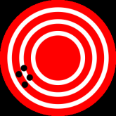
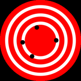
High accuracy and low precision (left) and low accuracy and high precision (right)
From: Accuracy and precision, Wikipedia, http://en.wikipedia.org/wiki/Accuracy_and_precision

To put that another way, when it comes to specific outcomes, the degree of accuracy is inversely proportional to the size of the system's event space (the scope across which the system is being observed). In terms of the system's performance patterns however, the degree of accuracy is directly proportional to the size of the system's event space.

One example would be the weather. The longer the time periods involved, the more accurate the forecast can be in terms of probable outcomes as patterns, but a specific event is virtually impossible to predict (such as rain at a certain place, a particular wind speed, etc). The smaller the event space (eg, standing at a certain spot over the next hour) the more accurate the prediction would be (for example, will it rain during the next few minutes). On the other hand, during a weather pattern representing a low pressure system for example, predictions can be made as to the likelihood of certain phenomena occurring which pertain to low pressure systems. And on a larger scale still, the likelihood of snow falling during summer is very low indeed (although it again depends on the overall set of probabilities defined by such parameters as latitude and elevation).

In the case of CauseF, using the same parameter settings will give different results every time (ascertainable through the cycle limits), but there will be a pattern in terms of the probability envelopes defined by the parameters.

CauseF also allows the user to observe the effects of self-adjusting probability levels, percentages that change as a consequence of outcomes during the cycles.

Sources and elements can be grouped into regions with their own specific probability levels as well as their own self-adjustment properties.

The maximum number of sources is set at Total number of units - 10.

Settings window

The Settings and Regions (element details) windows can be closed with the Esc key.

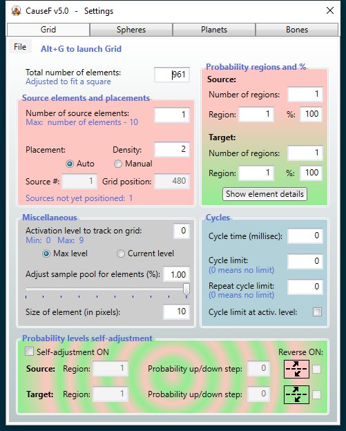
In order of appearance, left to right, top to bottom, by section:

(1) Total number of elements
The total number of elements the grid will contain. The number is adjusted to fit a square.

(2) Source elements and placements - Number of source elements
The number of sources. Can be no larger than Total number of elements - 10.

(3) Source elements and placements - Placement
Defines where in the entire grid the sources will be placed.

(4) Source elements and placements - Density
If (5) Auto is clicked, the sources will be placed symmetrically from the centre outwards with the selected Density defining how many squares in between.

(5) Source elements and placements - Auto
If selected, the sources will be placed symmetrically from the centre outwards with the selected Density defining how many squares in between.

(6) Source elements and placements - Manual
Sources will be placed according to (7) Source # and (8) Grid position.

(7) Source elements and placements - Source #
The ID number of a source, from 1 to Number of source elements.

(8) Source elements and placements - Grid position
The source's square number within the range given by Total number of elements.

(9) Probability regions and % - Source - Number of regions
Default is 1. If set to a number > 1 the total number of sources are split into groups (regions), where each region can be defined separately in terms of its (10) Region number and its (11) % probability level.

(10) Probability regions and % - Source - Region
The region number out of the (9) Probability regions and % - Source - Number of regions which is set to a certain (11) Probability regions and % - Source - % probability level.

(11) Probability regions and % - Source - %
The probability level assigned to (10) Probability regions and % - Source - Region. A level of 100% means all of the targets available can be accessed by that source. On the other hand, a 50% probability for example means the number range has been increased to double its size and the random number is selected from that pool, thereby giving the result a 50% chance of being one of the squares in the grid. With a 20% level the number range is increased to 5 times its size, and so on.

(12) Probability regions and % - Target - Number of regions
Default is 1. If set to a number > 1 the total number of targets are split into groups (regions), where each region can be defined separately in terms of its (13) Probability regions and % - Target - Region number and its (14) Probability regions and % - Target - % probability level.

(13) Probability regions and % - Target - Region
The region number out of the (12) Probability regions and % - Target - Number of regions which is set to a certain (14) Probability regions and % - Target - % probability level.

(14) Probability regions and % - Target - %
The probability level assigned to (12) Probability regions and % - Target - Region. A level of 100% means all of the targets available can be accessed by that temporary source (it's technically a target). On the other hand, a 50% probability for example means the number range has been increased to double its size and the random number is selected from that pool, thereby giving the result a 50% chance of being one of the squares in the grid. With a 20% level the number range is increased to 5 times its size, and so on.

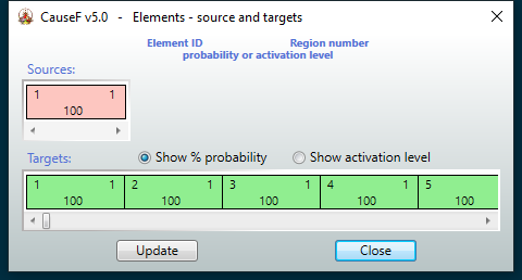
(15) Probability regions and % - Show element details
Brings up a window with the source and target regions arraigned next to each other, each element showing its ID, region number, and probability / activation level. Note that with more then 5000 elements (sources or targets) every 1000th is shown, with more than 50,000 every 10,000th is shown (prevents the display from taking too long).

(16) Miscellaneous - Activation level to track on grid
During cycling the number of elements at a certain activation level is displayed in the Grid window (see Grid window → (7) Max number of elem's at activation level *). With the default set to 0 the number of elements with activation level still at 0 is shown, if set to '1' the number of elements that have reached an activation level of 1 is shown, etc. It is one way to follow the progress of activations within the grid overall. The maximum is 9.

(17) Miscellaneous - Max level
If selected the total number of elements that have reached the activation level under (16) Miscellaneous - Activation level to track on grid in the Grid window is shown. There it is updated only when a new element has reached that activation level.

(18) Miscellaneous - Current level
When selected the current number of elements that have reached the activation level under (16) Miscellaneous - Activation level to track on grid in the Grid window is shown. There it is updated for every cycle.

(19) Miscellaneous - Adjust sample pool for elements (%)
Sets the percentage of the total number of target elements available to calculate their activation levels. The smaller this value the earlier any activation target will be reached. Useful for very large element numbers. Can be adjusted while the grid is cycling. Note: while it is not the same as adjusting the probability levels for sources and targets, the latter with their sample pools are a subset of that percentage.

(20) Miscellaneous - Size of element (in pixels)
Increases or decreases the size of the elements and thereby the entire grid. Note: the grid window can also be resized with the mouse. Resize the window slightly if the grid lines don't render properly (a window / monitor issue).

(21) Cycles - Cycle time (millisec)
Sets the time for one cycle. If 0, the time for each cycle is left to the system. If set to above 0, that time (in milliseconds) is added to each cycle's duration.

(22) Cycles - Cycle limit
If set to 0, the system will only stop cycling when Stop in the Grid window is clicked. Any value above 0 makes the system stop once that number of cycles has been reached. From then on clicking Start in the Grid window will advance the system by one cycle. Ineffective if (23) Cycles - Repeat cycle limit is set to a value above 0.

(23) Cycles - Repeat cycle limit
If set to any value above 0, the grid will advance by that many cycles every time Start in the Grid window is clicked.

(24) Cycles - Cycle limit at activ. level
If checked, the cycling will stop as soon as a target element has reached the activation level set at (16) Miscellaneous - Activation level to track on grid. Note that (17) Miscellaneous - Max level must be selected first.

(25) Probability levels self-adjustment - Self-adjustment ON
If checked the probability levels for a particular source and/or target region will be automatically adjusted according to the settings in this section.

(26) Probability levels self-adjustment - Source - Region
Sets the source region number for which probability steps are to be set.

(27) Probability levels self-adjustment - Source - Probability up/down step
Sets the value by which the probability level is set to adjust itself. If the probability level for that region is at 50% or above, at any time during cycling a source of that region will have its probability level incremented by that amount. If probability is below 50%, that source's probability level will be decremented by that amount. In effect the system will trend towards extremes.

(28) Probability levels self-adjustment - Source - Reverse ON
If checked, any probability level above 50% will step down towards 50%, and any level below 50% will step up towards 50%. Therefore the system will flatten around the 50% mark. The symbol next to it changes as below:
  → 

(29) Probability levels self-adjustment - Target - Region
Sets the target region number for which probability steps are to be set.

(30) Probability levels self-adjustment - Target - Probability up/down step
Sets the value by which the probability level is set to adjust itself. If the probability level for that region is at 50% or above, at any time during cycling a target of that region will have its probability level incremented by that amount. If probability is below 50%, that target's probability level will be decremented by that amount. In effect the system will trend towards extremes.

(31) Probability levels self-adjustment - Target - Reverse ON
If checked, any probability level above 50% will step down towards 50%, and any level below 50% will step up towards 50%. Therefore the system will flatten around the 50% mark. The symbol next to it changes as below:
  → 

Grid window

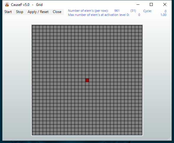
In order of appearance, left to right, top to bottom:

(1) Start
Starts the grid cycles. If disabled, click (3) Apply / Reset first.

(2) Stop
Stops the grid cycles. The grid remains in the current state.

(3) Apply / Reset
Applies the grid's parameters to the values defined under Settings → Grid, and/or resets them after they have changed during cycling.

(4) Close
Closes the Grid window. Cycling must be stopped first. Any parameter values as a result of cycling will be lost.

(5) Number of elem's (per row)
The total number of elements in the grid, includes sources and targets. The number in brackets refers to the number of elements (squares) per row.

(6) Cycle
The nth cycle performed by the system.

(7) Max number of elem's at activation level *
If (17) Miscellaneous - Max level in Grid window → Settings has been selected. It is updated only when a new element has reached that activation level. If (18) Miscellaneous - Current level has been selected the text changes to Current number of elem's at activation level *. '*' stands for the value defined in (16) Miscellaneous - Activation level to track on grid. It is updated for every cycle.

(8) Number on far right
The scalar applied to the percentage of the total number of target elements available to calculate their activation levels. Set under (19) Miscellaneous - Adjust sample pool for elements (%) in Settings. The smaller this value the earlier any activation target will be reached. Useful for very large element numbers. Can be adjusted while the grid is cycling. Note: while it is not the same as adjusting the probability levels for sources and targets, the latter with their sample pools are a subset of that percentage.

© Martin Wurzinger - see Terms of Use